When studying the basics of quantum computing we start describing circuits with easy calculations on 2×2 or 4×4 matrices, but as soon as we explore the first algorithms we stumble upon oracles that seem to be too complex to be represented like that. But matrices are very important for us developers: they are like functions that we can design and inspect regardless of the input. If we could describe any circuit as a simple combination of matrices, programming circuits would be similar to programming functions. There must be a way. Maybe I found one.
Let's start by importing the needed libraries and defining convenience functions to easily draw circuits and unitary matrices:
from qiskit import QuantumCircuit, execute, Aer
import math

def draw(circuit):
    return circuit.draw(output='mpl')

def unitary(circuit):
    unitary = execute(circuit, Aer.get_backend('unitary_simulator')).result().get_unitary()
    pretty_unitary = ''
    for row in range(len(unitary)):
        pretty_unitary += '|'
        for column in range(len(unitary[row])):
            value = unitary[row][column]
            if math.isclose(value.imag, 0, abs_tol=0.01):
                pretty_value = '{num.real:.0f}'.format(num=value)
            elif math.isclose(value.real, 0, abs_tol=0.01):
                pretty_value = '{num.imag:.0f}i'.format(num=value)
            else:
                pretty_value = '{num.real:.0f}+{num.imag:.0f}i'.format(num=value)

            pretty_unitary += pretty_value
            if column < len(unitary[row])-1:
                pretty_unitary += ' '
        pretty_unitary += '|\n'
    print(pretty_unitary)
Since we are going to deal with huge matrices, to make calculations simpler let's also define the following two "atomic" matrices:
0ˉ=∣0⟩⟨0∣=[1000]1ˉ=∣1⟩⟨1∣=[0001]
Their meaning is just "the current state of the qubit is ∣0⟩ (or ∣1⟩, respectively)."
Although these atoms are not reversible (e.g. 0ˉ⋅0ˉ†=0ˉ=I), they allow to easily define other matrices as a combination of them:
I=[1001]=[1000]+[0001]=0ˉ+1ˉCX=⎣⎢⎢⎢⎡1000000100100100⎦⎥⎥⎥⎤=[0ˉ1ˉ1ˉ0ˉ]=[0ˉ000ˉ]+[01ˉ1ˉ0]=I⊗0ˉ+X⊗1ˉ
Note how this last sum can be easily interpreted as: "The second qubit remains the same if the first qubit is ∣0⟩, but gets flipped if the first qubit is ∣1⟩." That's exactly the description of a CNOT gate! It looks like this representation makes circuits more intuitive to describe.
Not all matrices can be defined by those two atoms, for example:
X=[0110]=[0100]+[0010]=∣1⟩⟨0∣+∣0⟩⟨1∣
This suggests the presence of another pair of atoms, however for the sake of our calculations we can just keep small matrices such as I and X as they are, knowing that ∣1⟩⟨0∣ can be defined as X⋅0ˉ and ∣0⟩⟨1∣ as X⋅1ˉ.
Now we are able to describe all gates as a combination of 2×2 matrices, which means we can:
- Reverse-engineer huge unitary matrices by splitting them into atoms
- Describe circuits by defining each gate as a tensor product of atoms
- "Forward-engineer" circuits by describing the result we expect from them!
CNOT01
We know how the CNOT gate works on a two-qubits circuit. We expect no surprises if we add a (completely useless) third qubit.
circuit = QuantumCircuit(3)
circuit.cx(0, 1)
draw(circuit)
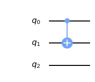
The corresponding unitary matrix should be pretty straightforward, we just need to treat the missing gate in q2 as an Identity matrix. Let's turn it into a combination of smaller matrices:
I⊗CX=[CX00CX]=⎣⎢⎢⎢⎡0ˉ1ˉ001ˉ0ˉ00000ˉ1ˉ001ˉ0ˉ⎦⎥⎥⎥⎤=⎣⎢⎢⎢⎡0ˉ00000ˉ00000ˉ00000ˉ⎦⎥⎥⎥⎤+⎣⎢⎢⎢⎡01ˉ001ˉ0000001ˉ001ˉ0⎦⎥⎥⎥⎤=I⊕I⊕0ˉ+I⊕X⊕1ˉ
Which we can interpret as: "q1 remains the same if q0 is equal to ∣0⟩, but gets flipped when it's ∣1⟩; q2 is irrelevant." This is exactly the same as describing a CNOT gate between q0 and q1, with an Identity matrix on q2!
unitary(circuit)
|1 0 0 0 0 0 0 0|
|0 0 0 1 0 0 0 0|
|0 0 1 0 0 0 0 0|
|0 1 0 0 0 0 0 0|
|0 0 0 0 1 0 0 0|
|0 0 0 0 0 0 0 1|
|0 0 0 0 0 0 1 0|
|0 0 0 0 0 1 0 0|
CNOT12
Nothing much changes if the third qubit is instead positioned on top, to be the first one.
circuit = QuantumCircuit(3)
circuit.cx(1, 2)
draw(circuit)
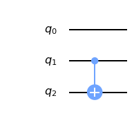
Here we can also easily calculate the resulting unitary matrix and split it into a combination of smaller matrices, just like before:
CX⊗I=⎣⎢⎢⎢⎡I000000I00I00I00⎦⎥⎥⎥⎤=⎣⎢⎢⎢⎡I000000000I00000⎦⎥⎥⎥⎤+⎣⎢⎢⎢⎡0000000I00000I00⎦⎥⎥⎥⎤=I⊗0ˉ⊗I+X⊗1ˉ⊗I
The interpretation is pretty similar to the previous, only the order changes: "q2 remains the same if q1 is equal to ∣0⟩, but gets flipped if q1 is ∣1⟩; q0 is irrelevant."
unitary(circuit)
|1 0 0 0 0 0 0 0|
|0 1 0 0 0 0 0 0|
|0 0 0 0 0 0 1 0|
|0 0 0 0 0 0 0 1|
|0 0 0 0 1 0 0 0|
|0 0 0 0 0 1 0 0|
|0 0 1 0 0 0 0 0|
|0 0 0 1 0 0 0 0|
CNOT02
circuit = QuantumCircuit(3)
circuit.cx(0, 2)
draw(circuit)
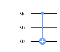
Here it gets trickier, because the I is between the control and the target of the CNOT. I have no idea how to build this matrix, so I'll leave this calculation to Qiskit:
unitary(circuit)
|1 0 0 0 0 0 0 0|
|0 0 0 0 0 1 0 0|
|0 0 1 0 0 0 0 0|
|0 0 0 0 0 0 0 1|
|0 0 0 0 1 0 0 0|
|0 1 0 0 0 0 0 0|
|0 0 0 0 0 0 1 0|
|0 0 0 1 0 0 0 0|
We can see this matrix as:
⎣⎢⎢⎢⎡0ˉ01ˉ000ˉ01ˉ1ˉ00ˉ001ˉ00ˉ⎦⎥⎥⎥⎤=⎣⎢⎢⎢⎡0ˉ00000ˉ00000ˉ00000ˉ⎦⎥⎥⎥⎤+⎣⎢⎢⎢⎡001ˉ00001ˉ1ˉ00001ˉ00⎦⎥⎥⎥⎤=I⊗I⊗0ˉ+X⊗I⊗1ˉ
Which could be interpreted as: "q2 remains the same if q0 is equal to ∣0⟩, but gets flipped when q0 is ∣1⟩; q1 is irrelevant." This is exactly like the previous two gates, but again in a different order!
Now that we know how to reverse-engineer a unitary matrix into a circuit, is it also possible to do the opposite, by describing the circuit as its constituent gates, or even intuitively "forward-engineer" a circuit into a matrix? Let's try it out with the oracles described in real case scenarios.
Quantum Teleportation: CNOT12⋅CNOT01
circuit = QuantumCircuit(3)
circuit.cx(1, 2)
circuit.cx(0, 1)
draw(circuit)
Let's describe this circuit gate by gate:
(I⊗I⊗0ˉ+I⊗X⊗1ˉ)⋅(I⊗0ˉ⊗I+X⊗1ˉ⊗I)
Once we perform the multiplication we get this result:
=I⊗0ˉ⊗0ˉ+X⊗1ˉ⊗0ˉ+I⊗X⋅0ˉ⊗1ˉ+X⊗X⋅1ˉ⊗1ˉ
An interpretation could be: "if q0 is ∣0⟩ then q2 depends solely on q1; if q0 is ∣1⟩ then q1 will flip and q2 will follow depending on the value of q1."
Note that adding Hadamard gates doens't add much to the result:
circuit = QuantumCircuit(3)
circuit.h(1)
circuit.cx(1, 2)
circuit.cx(0, 1)
circuit.h(0)
draw(circuit)
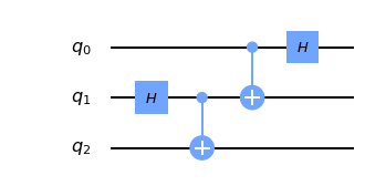
(I⊗I⊗H)⋅(I⊗I⊗0ˉ+I⊗X⊗1ˉ)⋅(I⊗0ˉ⊗I+X⊗1ˉ⊗I)⋅(I⊗H⊗I)
=I⊗0ˉ⋅H⊗H⋅0ˉ+X⊗1ˉ⋅H⊗H⋅0ˉ+I⊗X⋅0ˉ⋅H⊗H⋅1ˉ+X⊗X⋅1ˉ⋅H⊗H⋅1ˉ
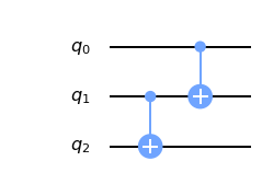
Deutsch-Josza: CNOT02⋅CNOT12
circuit = QuantumCircuit(3)
circuit.cx(0, 2)
circuit.cx(1, 2)
draw(circuit)
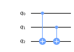
What does this circuit mean? How does it work? Let's reverse-engineer it by having a look at the computed unitary matrix:
unitary(circuit)
|1 0 0 0 0 0 0 0|
|0 0 0 0 0 1 0 0|
|0 0 0 0 0 0 1 0|
|0 0 0 1 0 0 0 0|
|0 0 0 0 1 0 0 0|
|0 1 0 0 0 0 0 0|
|0 0 1 0 0 0 0 0|
|0 0 0 0 0 0 0 1|
The matrix looks like the following:
⎣⎢⎢⎢⎡0ˉ01ˉ001ˉ00ˉ1ˉ00ˉ000ˉ01ˉ⎦⎥⎥⎥⎤=⎣⎢⎢⎢⎡0ˉ0000000ˉ000ˉ000ˉ00⎦⎥⎥⎥⎤+⎣⎢⎢⎢⎡001ˉ001ˉ001ˉ0000001ˉ⎦⎥⎥⎥⎤=CX⊗0ˉ+X⊗I⊗I⋅CX⊗1ˉ
Let's go a little further by expanding the CNOT gates:
=(I⊗0ˉ⊗0ˉ+X⊗1ˉ⊗0ˉ)+(X⊗I⊗I)⋅(I⊗0ˉ⊗1ˉ+X⊗1ˉ⊗1ˉ)
And now, applying the product:
=I⊗0ˉ⊗0ˉ+X⊗1ˉ⊗0ˉ+X⊗0ˉ⊗1ˉ+I⊗1ˉ⊗1ˉ
Which could be interpreted as: "q2 is flipped if only one of the other two is equal to ∣1⟩. In any other case it stays the same." It looks like a XOR which keeps the inputs in q0 and q1 and holds the output in q2. Now it makes sense!
Note that the result we found suggests to split the matrix in the following way, which is equivalent:
⎣⎢⎢⎢⎡0ˉ0000000000ˉ00000⎦⎥⎥⎥⎤+⎣⎢⎢⎢⎡00000000ˉ000000ˉ00⎦⎥⎥⎥⎤+⎣⎢⎢⎢⎡001ˉ000001ˉ0000000⎦⎥⎥⎥⎤+⎣⎢⎢⎢⎡000001ˉ0000000001ˉ⎦⎥⎥⎥⎤=⎣⎢⎢⎢⎡0ˉ01ˉ001ˉ00ˉ1ˉ00ˉ000ˉ01ˉ⎦⎥⎥⎥⎤
We could also describe the circuit as the sequence of its gates:
(I⊗0ˉ⊗I+X⊗1ˉ⊗I)⋅(I⊗I⊗0ˉ+X⊗I⊗1ˉ)
Now performing the multiplication:
=I⊗0ˉ⊗0ˉ+X⊗0ˉ⊗1ˉ+X⊗1ˉ⊗0ˉ+I⊗1ˉ⊗1ˉ
Which is exactly the result we got with reverse-engineering.
Simon: CNOT02⋅CNOT03⋅CNOT12⋅CNOT13
circuit = QuantumCircuit(4)
circuit.cx(0, 2)
circuit.cx(0, 3)
circuit.cx(1, 2)
circuit.cx(1, 3)
draw(circuit)
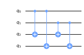
Let's try another "forward-engineer". The circuit could be descibed as:
- "q2 is flipped if q0 or q1 is ∣1⟩"
- "q3 is flipped if q0 or q1 is ∣1⟩"
- "Any other case doesn't change the state of "q2 or "q3"
Now, in maths:
1. (I⊗X⊗0ˉ⊗1ˉ)+(I⊗X⊗1ˉ⊗0ˉ)2. (X⊗I⊗0ˉ⊗1ˉ)+(X⊗I⊗1ˉ⊗0ˉ)3. (I⊗I⊗0ˉ⊗0ˉ)+(I⊗I⊗1ˉ⊗1ˉ)
We can simplify even further by combining 1. and 2. together, since both target qubits are flipped at the same time:
1+2. (X⊗X⊗0ˉ⊗1ˉ)+(X⊗X⊗1ˉ⊗0ˉ)3. (I⊗I⊗0ˉ⊗0ˉ)+(I⊗I⊗1ˉ⊗1ˉ)
If the description is correct, the resulting matrix should be:
⎣⎢⎢⎢⎢⎢⎢⎢⎢⎢⎢⎢⎡0000001ˉ000000000ˉ00001ˉ000000000ˉ00001ˉ000000000ˉ00001ˉ000000000ˉ000000⎦⎥⎥⎥⎥⎥⎥⎥⎥⎥⎥⎥⎤+⎣⎢⎢⎢⎢⎢⎢⎢⎢⎢⎢⎢⎡0ˉ000000001ˉ000000000ˉ000000001ˉ000000000ˉ000000001ˉ000000000ˉ000000001ˉ⎦⎥⎥⎥⎥⎥⎥⎥⎥⎥⎥⎥⎤=⎣⎢⎢⎢⎢⎢⎢⎢⎢⎢⎢⎢⎡0ˉ000001ˉ001ˉ000000ˉ000ˉ01ˉ0000001ˉ00ˉ00001ˉ00ˉ0000000ˉ01ˉ001ˉ000000ˉ000ˉ000001ˉ⎦⎥⎥⎥⎥⎥⎥⎥⎥⎥⎥⎥⎤
Will it work?
unitary(circuit)
|1 0 0 0 0 0 0 0 0 0 0 0 0 0 0 0|
|0 0 0 0 0 0 0 0 0 0 0 0 0 1 0 0|
|0 0 0 0 0 0 0 0 0 0 0 0 0 0 1 0|
|0 0 0 1 0 0 0 0 0 0 0 0 0 0 0 0|
|0 0 0 0 1 0 0 0 0 0 0 0 0 0 0 0|
|0 0 0 0 0 0 0 0 0 1 0 0 0 0 0 0|
|0 0 0 0 0 0 0 0 0 0 1 0 0 0 0 0|
|0 0 0 0 0 0 0 1 0 0 0 0 0 0 0 0|
|0 0 0 0 0 0 0 0 1 0 0 0 0 0 0 0|
|0 0 0 0 0 1 0 0 0 0 0 0 0 0 0 0|
|0 0 0 0 0 0 1 0 0 0 0 0 0 0 0 0|
|0 0 0 0 0 0 0 0 0 0 0 1 0 0 0 0|
|0 0 0 0 0 0 0 0 0 0 0 0 1 0 0 0|
|0 1 0 0 0 0 0 0 0 0 0 0 0 0 0 0|
|0 0 1 0 0 0 0 0 0 0 0 0 0 0 0 0|
|0 0 0 0 0 0 0 0 0 0 0 0 0 0 0 1|
It does! Now we are able to easily build and understand circuits, using just our common sense!
EDIT: I just stumbled upon a couple of answers on StackExchange which seem to get to the same conclusion for a question about the CNOT gate. Apparently they are referred to "algorithmic method" or "using projectors". There doesn't seem to be a standard though, I wonder why.
# IceOnFire


